Matrix Operations - Introduction#
Matrix operations are introduced to accompany the people who wants to use machine learning with GAMS or for people who prefer using matrix notation. In many machine-learning applications underlying algebra is written using matrix operations rather than using an indexed algebra. While GAMS provides indexed algebra to meet the demands of many common optimization applications, matrix operations are introduced to complement indexed algebra. We still think with the classical optimization problems indexed algebra is a better choice since it is more intuitive.
However for ML practitioners writing this:
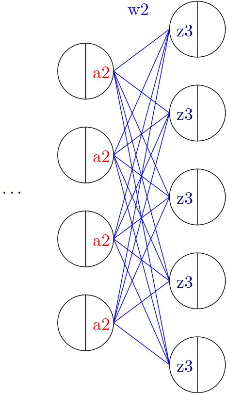
calc_mm_3[...] = z3 == a2 @ w2
is much easier than:
calc_mm_3[...] = z3[m, j] == Sum(k, a2[m, i] @ w2[i, j])
In this context, m represents the batch dimension, i denotes the feature dimension of layer 2, and j represents the feature dimension of layer 3.
GAMSPy provides the following features for ML workloads:
Implicit default domains
Easy matrix declaration
Matrix multiplication
- Convenience functions
Vector norms
Trace
Permute
Activation Functions
Improved domain tracking
In this introduction section, we summarize each of the features. You can find more information about the features in their own respective pages.
Implicit default domains#
GAMSPy can work without explicitly specifying the indices. Let a, b, c be variables (e.g. matrices). When symbols are accessed without specific domains, the domains specified when declaring the symbol is used implicitly.
import gamspy as gp
import numpy as np
m = gp.Container()
i = gp.Set(m, "i")
j = gp.Set(m, "j")
k = gp.Set(m, "k")

a = gp.Variable(m, name="a", domain=[i, j, k])
b = gp.Variable(m, name="b", domain=[j, k])
c = gp.Variable(m, name="c", domain=[i, j])
assign_1 = gp.Equation(m, name="assign_1", domain=[i, j, k])
The following expression works without specifying the indices:
assign_1[...] = a == b + c
If you prefer ellipsis syntax:
assign_1[...] = a[...] == b[...] + c[...]
Or if you want to be specific:
assign_1[...] = a[i, j, k] == b[j, k] + c[i, j]
Easy matrix declaration#
Sometimes you need to generate parameters or variables as a matrix and do not
put too much meaning to its indices. gp.math.dim function is our suggested
method for declaring matrices, however parameters or variables defined without
using it still can be used in matrix operations.
See the following example for using dim function:
import gamspy as gp
import numpy as np
from gamspy.math import dim

w1_data = np.random.rand(50, 100)
m = gp.Container()
w = gp.Parameter(m, name="w1", domain=dim((50, 100)), records=w1_data)
w.records
Output:
     DenseDim50_1 DenseDim100_1     value
0               0             0  0.429909
1               0             1  0.831080
2               0             2  0.656872
3               0             3  0.959341
4               0             4  0.758202
...           ...           ...       ...
4995           49            95  0.847640
4996           49            96  0.870642
4997           49            97  0.369344
4998           49            98  0.233120
4999           49            99  0.704139
As you can see under the hood, GAMSPy generates two sets for you called
DenseDim50_1 and DenseDim100_1. DenseDim50_1 contains elements
0, 1, ..., 49 whereas DenseDim100_1 contains elements
0, 1, ..., 99. The word DenseDim is followed by the dimension,
underscore and then the alias number where 1 refering the original set.
...
w2_data = np.random.rand(50, 50)
w2 = gp.Parameter(m, name="w2", domain=dim((50, 50)), records=w2_data)
w2.records
Output:
     DenseDim50_1 DenseDim50_2     value
0               0            0  0.902650
1               0            1  0.268446
2               0            2  0.133204
3               0            3  0.931026
4               0            4  0.283675
...           ...          ...       ...
2495           49           45  0.931849
2496           49           46  0.991170
2497           49           47  0.754725
2498           49           48  0.924075
2499           49           49  0.437851
You can see in the output DenseDim50_2 is used instead of repeating
the same set twice. DenseDim50_2 is an alias of set DenseDim50_1.
This is done because it is more convenient for us when doing matrix
multiplications.
In the same way you can generate variable matrices:
...
x = gp.Variable(m, name="x", domain=dim((50, 50)))
You are not limited to 2 dimensions. Many times in ML applications we need more than 2 dimensions:
...
y = gp.Variable(m, name="y", domain=dim((128, 500, 1000)))
However, you are limited to 20 dimensions as GAMS supports up to 20 dimensions:
...
# The following would not work
z = gp.Variable(m, name="z", domain=dim(list(range(1, 100))))
Matrix Multiplication#
We tried to follow matrix multiplication rules of PyTorch,
torch.matmul ,
therefore, you are not limited to only rank-2 tensor multiplications. GAMSPy
symbols and expressions support matrix multiplication by overriding @ operator.
Information
When performing matrix multiplication, the actual computation is not carried out immediately. Instead, an expression is generated. This approach is taken because matrix multiplication is computationally expensive, and since the elements involved include variables in addition to numbers, certain libraries and optimization techniques cannot be used to accelerate the process. By delegating this task to GAMS rather than handling it directly in Python, we achieve a faster model generation experience.
Validation of dimensions and shape of the output is determined by dimensions of the tensors as follows:
If both tensors are vectors, the dot product is returned.
If both tensors are matrices, matrix multiplication is returned.
If the first tensor is a vector and the second tensor is a matrix then 1 is prepended to the vector to make it a matrix multiplication. After the operation, the prepended dimension is removed.
If the first tensor is a matrix, and the second tensor is a vector, matrix-vector product is returned.
If the first tensor is a vector, and the second tensor has a rank larger than 2, the first tensor is prepended with 1 and then batched matrix multiplication is returned. After the operation, the prepended dimension is removed.
If the first tensor has a rank larger than 2, and the second tensor is a vector, then batched matrix-vector product is returned.
If both tensors have ranks larger than 2, then they must have same ranks. We currently do not support broadcasting. Batch dimensions must match.
You can see every case in the following example:
import gamspy as gp
import numpy as np
from gamspy.math import dim

# since we will use this a lot
rand = np.random.rand

m = gp.Container()
# inputs
vec  = gp.Parameter(m, name="vec",  domain=dim((25,   )), records=rand(25))
mat  = gp.Parameter(m, name="mat",  domain=dim((25, 25)), records=rand(25, 25))
mat2 = gp.Parameter(m, name="mat2", domain=dim((40, 50)), records=rand(40, 50))
mat3 = gp.Parameter(m, name="mat3", domain=dim((50, 60)), records=rand(50, 60))

# case 1: vector @ vector, dot product
f = gp.Parameter(m, name="f")
f[...] = vec @ vec
print(f"{f.records=}")
# 0  9.181418

# case 2: matrix @ matrix, matrix multiplication
# 40 by 50 times 50 by 60 resulting in 40 by 60
res_mat = gp.Parameter(m, name="res_mat", domain=dim((40, 60)))
res_mat[...] = mat2 @ mat3
print(f"{res_mat.records}")
#     DenseDim40_1 DenseDim60_1      value
#0               0            0   8.648533
#1               0            1  10.884543
#2               0            2  10.512125
#3               0            3  10.892082
#4               0            4   9.390584
#...           ...          ...        ...
#2395           39           55  13.436246
#2396           39           56  12.606727
#2397           39           57  12.442652
#2398           39           58  12.599677
#2399           39           59  12.669896

# case 3: vector @ matrix
res_vec = gp.Parameter(m, name="res_vec", domain=dim((25,)))
res_vec[...] = vec @ mat

# case 4: matrix @ vector
res_vec[...] = mat @ vec

# case 5: vector @ batched matrix
# 20 times 128x20x90
# vector is prepended by 1
# 1x20 times 128x20x90
# resulting in 128x90
vec_2 = gp.Parameter(m, name="vec_2", domain=dim((20,)), records=rand(20))
batched_mat = gp.Parameter(m, name="batched_mat",
                           domain=dim((128, 20, 90)), records=rand(128, 20, 90))
result_mat = gp.Parameter(m, name="result_mat", domain=dim((128, 90)))
result_mat[...] = vec_2 @ batched_mat

# case 6: batched matrix @ vector
vec_3 = gp.Parameter(m, name="vec_3", domain=dim((90,)), records=rand(90))
result_mat_2 = gp.Parameter(m, name="result_mat_2", domain=dim((128, 20)))
result_mat_2[...] = batched_mat @ vec_3

# case 7: batched matrix @ batched matrix
batched_mat_2 = gp.Parameter(m, name="batched_mat_2",
                             domain=dim((128, 90, 50)), records=rand(128, 90, 50))
result_mat_3 = gp.Parameter(m, name="result_mat_3", domain=dim((128, 20, 50)))
result_mat_3[...] = batched_mat @ batched_mat_2
Convenience Functions#
Similar to matrix multiplications, there exist many mathematical functions that are frequently used in machine learning applications.
Vector Norms#
Vector norms are essential to many machine learning applications. For example, in ordinary least squares method, one minimizes the squared residuals which can be formulated as minimizing the vector size of the residuals.
In the simple example, we can use vector_norm
to get length of a vector.
import gamspy as gp
import numpy as np
from gamspy.math import vector_norm

m = gp.Container()
i = gp.Set(m, name="i", records=["i1", "i2"])
# (3, 4) vector
vec = gp.Parameter(m, "vec", domain=[i], records=[("i1", 3), ("i2", 4)])
# Size of a vector is a scalar
vlen = gp.Parameter(m, "vlen", domain=[])
vlen[...] = gp.math.vector_norm(vec)
vlen.records
#    value
# 0    5.0
The vector_norm function calculates the Euclidean norm of an input by default, flattening all dimensions. It can also compute any Lp-norm with some considerations:
Default Behavior: Without additional arguments, the function returns the Euclidean norm.
Custom Lp-norm: To calculate an Lp-norm, supply the desired value of ord.
Special Case: If ord is not an even integer and the input is not an endogenous argument, the norm calculation uses the absolute value, which requires DNLP.
You can also use dim function to specify over which dimensions to compute the norm.
import gamspy as gp
import numpy as np
from gamspy.math import vector_norm

m = gp.Container()
i = gp.Set(m, name="i", records=["i1", "i2"])
j = gp.Set(m, name="j", records=["j1", "j2"])
mat = gp.Parameter(m, "mat", domain=[i, j],
                   records=[
                     ("i1", "j1", 3),
                     ("i1", "j2", 4),
                     ("i2", "j1", 7),
                     ("i2", "j2", 24),
                   ]
                  )
vlen = gp.Parameter(m, "vlen", domain=[i])
vlen[...] = gp.math.vector_norm(mat, dim=[j])
vlen.records
#     i  value
# 0  i1    5.0
# 1  i2   25.0
Canceling out the square root#
It is common to minimize the L2 norms of residuals in optimization problems. Minimizing an L2 norm typically requires using the square root (sqrt) function, which necessitates using a Non-Linear Programming (NLP) model type. However, in many cases, you can achieve this by minimizing the square of the norm instead, allowing the use of a Quadratically Constrained Programming (QCP) model type.
Normally, this approach wouldn’t work in GAMSPy because the square and square
root operations do not cancel each other automatically. However, the
vector_norm operation is an exception. When the conditions are correct,
vector_norm marks the sqrt
function as cancellable, effectively allowing the minimization of the squared
norm within a QCP model.
This enhanced functionality simplifies the optimization process and broadens the applicability of the vector_norm function in various modeling scenarios.
import gamspy as gp
import numpy as np
from gamspy.math import vector_norm

m = gp.Container()
i = gp.Set(m, name="i", records=["i1", "i2"])
j = gp.Set(m, name="j", records=["j1", "j2"])
mat = gp.Parameter(m, "mat", domain=[i, j],
                   records=[
                     ("i1", "j1", 3),
                     ("i1", "j2", 4),
                     ("i2", "j1", 7),
                     ("i2", "j2", 24),
                   ]
                  )
expr = gp.math.vector_norm(mat, dim=[j])
expr.gamsRepr()
# '( sqrt(sum(j,( sqr(mat(i,j)) ))) )'

# You can see square cancels the square root in this case
(expr ** 2).gamsRepr()
# 'sum(j,( sqr(mat(i,j)) ))'
Permute#
Another very common operation that is often required is permutation. The
permute function takes an input x and dims
where the x is one of the following:
Parameter
ImplicitParameter
Variable
ImplicitVariable
and returns either an ImplicitVariable or ImplicitParameter where the dimensions are permuted as requested.
permute does not create a new variable or parameter in GAMS but rather creates a placeholder when accesed doing the permutation and accessing the original variable. You can see that in the following example we create a matrix mat with domain [i, j]. Afterwards, we set mat2 to a permutation of the mat but printing the GAMS string of mat2 reveals that no new variable is generated.
import gamspy as gp
import numpy as np
from gamspy.math import permute

m = gp.Container()
i = gp.Set(m, name="i", records=["i1", "i2"])
j = gp.Set(m, name="j", records=["j1", "j2"])
mat = gp.Parameter(m, "mat", domain=[i, j],
                   records=[
                     ("i1", "j1", 3),
                     ("i1", "j2", 4),
                     ("i2", "j1", 7),
                     ("i2", "j2", 24),
                   ]
                  )

mat2 = permute(mat, [1, 0])
mat2.gamsRepr()
# 'mat(i,j)'
mat2.domain
# [<Set `j` (0x...)>, <Set `i` (0x...)>]

mat2["i1", "j2"] # This would raise an exception

mat2["j2", "i2"] # This is the correct way to reach mat2

mat2["j2", "i2"].gamsRepr()
# 'mat("i1","j2")'
If you need to just permute last two dimensions, aka transpose, you can use .t() on parameters and variables.
import gamspy as gp
import numpy as np

m = gp.Container()
i = gp.Set(m, name="i", records=["i1", "i2"])
j = gp.Set(m, name="j", records=["j1", "j2"])
mat = gp.Parameter(m, "mat", domain=[i, j],
                   records=[
                     ("i1", "j1", 3),
                     ("i1", "j2", 4),
                     ("i2", "j1", 7),
                     ("i2", "j2", 24),
                   ]
                  )

mat2 = mat.t() # same as before
Trace#
The trace function calculates the trace of a given
input array x. Although less common in machine learning, this function can
still be useful in various applications.
Default Behavior: By default, the function computes the trace along the zeroth and first axes.
Custom Axes: Use the axis1 and axis2 parameters to specify different axes for the trace calculation. The domains of axis1 and axis2 must be the same or aliases.
import gamspy as gp
import numpy as np
from gamspy.math import trace

m = gp.Container()
i = gp.Set(m, name="i", records=["i1", "i2"])
# Matrix
# 3 4
# 5 6
# Trace of it is 3 + 6 = 9

mat = gp.Parameter(m, "mat", domain=[i, i],
                   records=[
                     ("i1", "i1", 3),
                     ("i1", "i2", 4),
                     ("i2", "i1", 5),
                     ("i2", "i2", 6),
                   ]
                  )

sc = gp.Parameter(m, name="sc", domain=[])
sc[...] = trace(mat)
sc.records
#    value
# 0    9.0
Activation Functions#
One of the key reasons neural networks can learn a wide range of tasks is their ability to approximate complex functions, including non-linear ones. Activation functions are essential components that introduce non-linearity to neural networks. While understanding functions like ReLU may be straightforward, integrating them into optimization models can be challenging. To assist you, we have started with a small list of commonly used activation functions. So far, we have implemented the following activation functions:
Unlike other mathematical functions, these activation functions return a
variable instead of an expression. This is because ReLU cannot be represented
with a single expression. Directly writing y = max(x, 0) without reformulating
it would result in a Discontinuous Nonlinear Program (DNLP) model, which is
highly undesirable. Currently, you can either use
relu_with_binary_var to
introduce binary variables into your problem, or
relu_with_complementarity_var
to introduce nonlinearity.
Your model class changes based on whether you want to embed a pre-trained neural network into your problem or train a neural network within your problem.
If you are training a neural network, you must have non-linearity. Using
relu_with_binary_var
would result in a Mixed-Integer Nonlinear Program (MINLP) model. On the other
hand, relu_with_complementarity_var
would keep the model as a Nonlinear Program (NLP) model, though this does not
necessarily mean it will train faster.
If you are embedding a pre-trained neural network using
relu_with_binary_var,
you can maintain your model as a Mixed-Integer Programming (MIP) model,
provided you do not introduce nonlinearities elsewhere.
To read more about classification of models.
from gamspy import Container, Variable, Set
from gamspy.math import relu_with_binary_var, log_softmax
from gamspy.math import dim


batch = 128
m = Container()
x = Variable(m, "x", domain=dim([batch, 10]))
y = relu_with_binary_var(x)

y2 = log_softmax(x) # this creates variable and equations for you
Additionally, we offer our established functions that can also be used as activation functions:
These functions return expressions like the other math functions. So, you need to create equations and variables yourself.
from gamspy import Container, Variable, Set, Equation
from gamspy.math import dim, tanh


batch = 128
m = Container()
x = Variable(m, "x", domain=dim([batch, 10]))
eq = Equation(m, "set_y", domain=dim([batch, 10]))
y = Variable(m, "y", domain=dim([batch, 10]))
eq[...] = y == tanh(x)
Improved domain tracking#
GAMSPy provides a flexible implementation of matrix multiplication that goes beyond parameters and variables. Expressions can also be used within matrix multiplications. To support this functionality, GAMSPy tracks the domain of each expression.
You can query the domain of an expression by using the domain attibute. In some cases, in addition to tracking the domain, GAMSPy needs to change domain in order to preserve domains when the resulting multiplication has the same set in its domain more than once. You can also use this feature to change a set or alias to its alias. You can see the following code snippet for the example.
import gamspy as gp
import numpy as np
m = gp.Container()
i = gp.Set(m, "i")
j = gp.Set(m, "j")
k = gp.Set(m, "k")

a = gp.Variable(m, name="a", domain=[i, j])
b = gp.Variable(m, name="b", domain=[k, j])
c = gp.Variable(m, name="c", domain=[i, k])

expr = a + b
expr.domain
# [<Set `i` (0x...)>, <Set `j` (0x...)>, <Set `k` (0x...)>]

expr2 = c + b
expr2.domain
# [<Set `i` (0x...)>, <Set `k` (0x...)>, <Set `j` (0x...)>]


expr3 = expr @ expr2
expr3.domain
# [<Set `i` (0x...)>, <Alias `AliasOfj_2` (0x...)>, <Set `j` (0x...)>]
expr3.gamsRepr()
# 'sum(k,((a(i,AliasOfj_2) + b(k,AliasOfj_2)) * (c(i,k) + b(k,j))))'

# if you want to use your own alias
jj = gp.Alias(m, "jj", j)
expr4 = expr3[i, jj, j]
expr4.gamsRepr()
# 'sum(k,((a(i,jj) + b(k,jj)) * (c(i,k) + b(k,j))))'