Binary Classification Example#
Learning to classify between 2 (or more) classes is a common problem that can arise from many real life applications. For example, you might have some traffic data and you can try to learn depending on some parameters if some road is congested or not. Depending on how many hours studied, you can try to learn if a student will fail or pass.
One of the most common techniques to handle binary classification problems is so-called logistic regression approach.
To learn more about Logistic Regression.
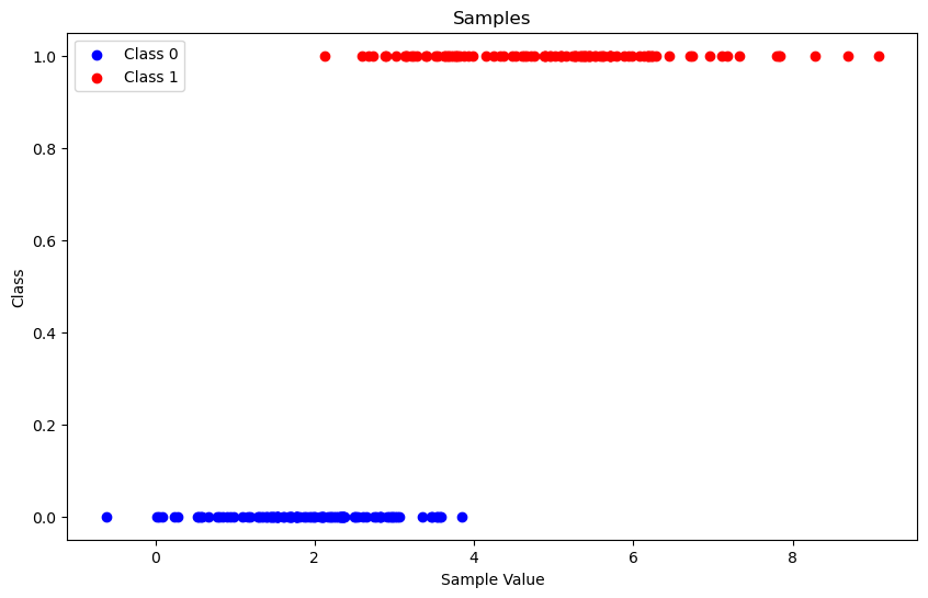
We start with generating a simple dataset. We have a single feature, and two gaussian distributions where class 1 and class 2 are sampled from.
import numpy as np
import matplotlib.pyplot as plt

np.random.seed(42)

num_samples = 100

# Parameters for the first Gaussian distribution
mean1 = 2.0
std_dev1 = 1.0

# Parameters for the second Gaussian distribution
mean2 = 5.0
std_dev2 = 1.5

# Generate samples
samples0 = np.random.normal(mean1, std_dev1, num_samples)
samples1 = np.random.normal(mean2, std_dev2, num_samples)

# Plot the samples
plt.figure(figsize=(10, 6))
plt.scatter(samples0, np.zeros_like(samples0), color='blue', label='Class 0')
plt.scatter(samples1, np.zeros_like(samples1) + 1, color='red', label='Class 1')
plt.xlabel('Sample Value')
plt.ylabel('Class')
plt.title('Samples')
plt.legend()
plt.show()
Our goal is to fit parameters of a function (yes, the logistic function) where we input the feature of a sample, we calculate the probability of this sample belonging to class 1. Since we have only two classes, 1 minus that probability will give us the probability of that sample belonging to class 0.
Just by looking at the samples, you can guess \(f(0)\) should be very close to 0 whereas \(f(8)\) should be close to 1.
The function that we are trying to fit is:
We need to come-up with \(\beta_0\) and \(\beta_1\) values so that samples belonging to class 1 have a higher \(p(x)\) and samples belonging to class 0 have \(p(x)\) close to 0.
Let’s start with passing data to GAMSPy
import gamspy as gp
import sys
from gamspy.math import dim, exp, log

m = gp.Container()

class_0_samples = gp.Parameter(m, name="samples_0",
                               domain=dim([100]), records=samples0)

class_1_samples = gp.Parameter(m, name="samples_1",
                               domain=dim([100]), records=samples1)

dim_100 = class_0_samples.domain[0]
Then, we are searching to optimize coefficients \(\beta_0\) and \(\beta_1\) minimizing the loss.
b0 = gp.Variable(m, name="bias")
b1 = gp.Variable(m, name="coefficient")
loss = gp.Variable(m, name="loss")
We are using the log loss for guiding our optimization, which you can read more from the wikipedia article we cited.
def logistic(c0, c1, x):
    return 1 / (1 + exp(-c0 - x * c1))


def_loss = gp.Equation(m, name="calc_loss")

# Define the loss function
def_loss[...] = loss == gp.Sum(dim_100, - log(logistic(b0, b1, class_1_samples[...]))) + \
            gp.Sum(dim_100, - log(1 - logistic(b0, b1, class_0_samples[...])))
This is basically all we need, we put everything under logistic model and solve it using your favourite NLP solver.
model_logistic = gp.Model(
        m,
        name="logistic",
        equations=m.getEquations(),
        problem="NLP",
        sense="min",
        objective=loss,
)

model_logistic.solve() # output=sys.stdout if you like to show the log from the solver

class_1_accuracy = gp.Parameter(m, name="accuracy1")
class_1_accuracy[...] = gp.Sum(dim_100, logistic(b0.l,  b1.l, class_1_samples) >= 0.5)


class_0_accuracy = gp.Parameter(m, name="accuracy2")
class_0_accuracy[...] = gp.Sum(dim_100, logistic(b0.l,  b1.l, class_0_samples) < 0.5)

learned_b0 = b0.toDense()
learned_b1 = b1.toDense()

avg_accuracy = (class_1_accuracy.toDense() + class_0_accuracy.toDense()) / 2
print(avg_accuracy, "% Accuracy")
# 91.0 % Accuracy
If we plot the logistic function on top of the samples:
def predict_class(b0, b1, x):
    prob = 1 / (1 + np.exp(-b0 - x * b1))
    return prob


# Create labels for the samples
labels1 = np.ones(100)
labels0 = np.zeros(100)

# Combine samples and labels
X = np.concatenate((samples1, samples0)).reshape(-1, 1)
y = np.concatenate((labels1, labels0))


# Generate a range of values for plotting the logistic function
x_values = np.linspace(min(X), max(X), 500).reshape(-1, 1)
y_values = predict_class(learned_b0, learned_b1, x_values)


plt.figure(figsize=(10, 6))
plt.scatter(samples1, np.zeros_like(samples1) + 1, color='red')
plt.scatter(samples0, np.zeros_like(samples0), color='blue')

plt.plot(x_values, y_values, color='green', linewidth=2, label='Logistic Function')
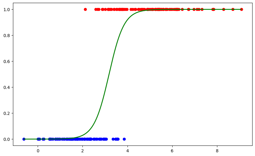
You can see how nicely the function is fitted over the samples. In this example, we only trained a logistic regression model but it is also possible to use this trained model in your optimization models.