Quick Start Guide#
![]()
Introduction#
This quick start guide is designed to provide you with a concise overview of GAMSPy and its key features. By the end of this guide, you’ll have a solid understanding of how to create basic mathematical models using GAMSPy. For more advanced features, we recommend exploring our comprehensive user guide and the extensive model library.
While not mandatory, having a basic understanding of Python programming and familiarity with the Pandas library will be helpful for following this tutorial.
A Transportation Problem#
In this guide, we’ll delve into an example of the transportation problem. This classic scenario involves managing supplies from various plants to meet demands at multiple markets for a single commodity. Additionally, we have the unit costs associated with shipping the commodity from plants to markets. The fundamental economic question here is:
How can we optimize the shipment quantities between each plant and market to minimize the total transport cost?
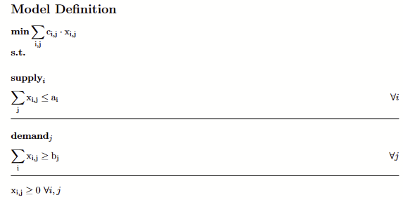
The problem’s algebraic representation typically takes the following format:
Indices (Sets):
\(i\) = plants
\(j\) = markets
Given Data (Parameters):
\(a_i\) = supply of commodity at plant \(i\) (in cases)
\(b_j\) = demand for commodity at market \(j\) (in cases)
\(c_{ij}\) = cost per unit of shipment between plant \(i\) and market \(j\)
Decision Variables:
\(x_{ij}\) = amount of commodity to ship from plant \(i\) to market \(j\) where \(x_{ij} \ge 0\) for all \(i,j\)
Constraints:
Observe supply limit at plant \(i\): \(\sum_j x_{ij} \le a_i \: \forall i\)
Satisfy demand at market \(j\): \(\sum_i x_{ij} \ge b_j \: \forall j\)
Objective Function: Minimize \(\sum_i \sum_j c_{ij} \cdot x_{ij}\)
Symbol Declaration#
In line with our systematic breakdown of the transportation problem into sets, parameters, variables, and constraints, we will adopt a similar approach to define the problem as a GAMSPy Model. To do so, it is essential to import the gamspy library initially.
[1]:
from gamspy import Container, Set, Parameter, Variable, Equation, Model, Sum, Sense, Options
Container#
Before we proceed further, let’s create a Container to encapsulate all the relevant information for our GAMSPy Model. This Container acts as a centralized hub, gathering essential data, sets, parameters, variables, and constraints, providing a clear structure for our optimization problem.
[2]:
m = Container()
Sets#
Sets serve as the fundamental building blocks of a GAMSPy Model, directly corresponding to the indices in the algebraic representations of models. In our transportation problem context, we have defined the following indices:
\(i\) = plants
\(j\) = markets
For detailed guidance on using sets, please refer to the set section of our user guide.
[3]:
i = Set(container=m, name="i", description="plants")
j = Set(container=m, name="j", description="markets")
i.name, j.name
[3]:
('i', 'j')
The effect of using the above Set statements is that we declared two sets, namely \(i\) and \(j\). Additionally, we provided descriptions to elaborate on their meaning, enhancing the readability of our Model. name argument of symbol constructors is optional. If the name is not provided, GAMSPy will generate a name for it automatically. Example of a symbol with an autogenerated name:
[4]:
dummy_symbol = Set(container=m)
dummy_symbol.name
[4]:
'dummy_symbol'
Providing a name to a symbol is highly recommended for many purposes. For example, if you want to reach to the symbol object via Container later in your script, you can get it with container['your_symbol_name']. It is also important for interoperability which will be explained later.
Parameters#
Parameters are declared using the Parameter class. Each parameter is assigned a name and a description. Note that parameter \(a_i\) is indexed by \(i\). To accommodate these indices, we include the domain attribute, pointing to the corresponding set.
[5]:
a = Parameter(
    container=m,
    name="a",
    domain=i,
    description="supply of commodity at plant i (in cases)"
)
b = Parameter(
    container=m,
    name="b",
    domain=j,
    description="demand for commodity at market j (in cases)"
)
c = Parameter(
    container=m,
    name="c",
    domain=[i, j],
    description="cost per unit of shipment between plant i and market j",
)
Variables#
GAMSPy variables are declared using Variable. Each Variable is assigned a name, a domain if necessary, a type, and, optionally, a description.
[6]:
x = Variable(
    container=m,
    name="x",
    domain=[i, j],
    type="Positive",
    description="amount of commodity to ship from plant i to market j",
)
This statement results in the declaration of a shipment variable for each (i,j) pair.
More information on variables can be found in the variable section of our user guide.
Equations#
A GAMSPy Equation can be declared and defined in two separate statements (see here how to do this in one statement). The format of the declaration is the same as for other GAMSPy symbols. First comes the keyword, Equation in this case, followed by the name, domain and text. The transportation problem has two constraints:
Supply: observe supply limit at plant \(i\): \(\sum_j x_{ij} \le a_i \: \forall i\)
Demand: satisfy demand at market \(j\): \(\sum_i x_{ij} \ge b_j \: \forall j\)
[7]:
supply = Equation(
    container=m, name="supply", domain=i, description="observe supply limit at plant i"
)
demand = Equation(
    container=m, name="demand", domain=j, description="satisfy demand at market j"
)
The components of an Equation definition are:
The Python variable of the
Equationbeing definedThe domain (optional)
Domain restricting conditions (optional)
A
=signLeft hand side expression
Relational operator (
==,<=,>=)The right hand side expression.
The Equation definition for the supply constraint of the transportation problem is implemented as follows:
[8]:
supply[i] = Sum(j, x[i, j]) <= a[i]
Using the same logic as above, we can define the demand equation as follows:
[9]:
demand[j] = Sum(i, x[i, j]) >= b[j]
The LaTeX representation of the equation can be retrieved with equation.latexRepr()
[10]:
print(demand.latexRepr())
$
\sum_{i} x_{i,j} \geq b_{j}\hfill \forall j
$
\begin{equation*} \sum_{i} x_{i,j} \geq b_{j}\qquad \forall j \end{equation*}
More information on equations is given in the equation section of our user guide.
Objective#
The objective function of a GAMSPy Model does not require a separate Equation declaration. You can either assign the objective expression to a Python variable or use it directly in the Model() statement of the next section. An alternative way of declaring the objective with a seperate Equation would look like the following:
[11]:
obj = Sum((i, j), c[i, j] * x[i, j])
Model#
A GAMSPy Model() consolidates constraints, an objective function, a sense (minimize, maximize, and feasibility), and a problem type. It also possesses a name and is associated with a Container.
To define our transportation problem as a GAMSPy Model, we assign it to a Python variable, link it to our Container (populated with symbols and data), name it “transport”, specify the equations, set the problem type as linear program (LP), specify the sense of the objective function (Sense.MIN), and point to the objective expression.
GAMSPy allows two alternatives to assign equations to a Model:
Using a list of equations,
Retrieving all equations by calling
m.getEquations().
Using a List of Equations#
Using a list of equations is especially useful if you want to define multiple GAMSPy Models with a subset of the equations in your Container. For the transportation problem this can be done as follows:
[12]:
transport = Model(
    m,
    name="transport",
    equations=[supply, demand],
    problem="LP",
    sense=Sense.MIN,
    objective=obj,
)
Retrieving all Equations#
Using m.getEquations() is especially convenient if you want to include all equations of your Container to be associated with your model. For the transportation problem this can be done as follows:
[13]:
transport = Model(
    m,
    name="transport",
    equations=m.getEquations(),
    problem="LP",
    sense=Sense.MIN,
    objective=obj,
)
More information on the usage of a GAMSPy Model can be found in the model section of our user guide.
Data#
Before solving our model, let’s set the data of the model using either Python primitives (i.e. list, tuple etc.) or the Pandas library. We’ll begin by organizing the necessary information, which we will subsequently feed into our optimization model. There are two ways to declare symbols:
Separate declaration and data assignment
Combine declaration and data assignment
[14]:
i.setRecords(['seattle', 'san-diego'])
j.setRecords(['new-york', 'chicago', 'topeka'])
a.setRecords([("seattle", 350), ("san-diego", 600)])
b.setRecords([("new-york", 325), ("chicago", 300), ("topeka", 275)])
i.records
[14]:
| uni | element_text | |
|---|---|---|
| 0 | seattle | |
| 1 | san-diego |
We assigned members to the sets, establishing a clear connection between the abstract sets and their real-world counterparts.
\(i\) = {Seattle, San Diego}
\(j\) = {New York, Chicago, Topeka}
To verify the content of a set, you can use <set name>.records.
[15]:
import pandas as pd

distances = pd.DataFrame(
    [
        ["seattle", "new-york", 2.5],
        ["seattle", "chicago", 1.7],
        ["seattle", "topeka", 1.8],
        ["san-diego", "new-york", 2.5],
        ["san-diego", "chicago", 1.8],
        ["san-diego", "topeka", 1.4],
    ],
    columns=["from", "to", "distance"]
).set_index(["from", "to"])
d = Parameter(
    container=m,
    name="d",
    domain=[i, j],
    description="distance between plant i and market j",
    records=distances.reset_index(),
)
d.records
[15]:
| from | to | value | |
|---|---|---|---|
| 0 | seattle | new-york | 2.5 |
| 1 | seattle | chicago | 1.7 |
| 2 | seattle | topeka | 1.8 |
| 3 | san-diego | new-york | 2.5 |
| 4 | san-diego | chicago | 1.8 |
| 5 | san-diego | topeka | 1.4 |
The cost per unit of shipment between plant \(i\) and market \(j\) is derived from the distance between \(i\) and \(j\) and can be calculated as follows:
\(c_{ij} = \frac{90 \cdot d_{ij}}{1000}\),
where \(d_{ij}\) denotes the distance between \(i\) and \(j\).
We have two options to calculate \(c_{ij}\) and assign the data to the GAMSPy parameter:
Python assignment - calculation in Python, e.g., using Pandas and
<parameter name>.setRecords()GAMSPy assignment - calculation in GAMSPy
[16]:
freight_cost = 90
cost = freight_cost * distances / 1000
c.setRecords(cost.reset_index())
c.records
[16]:
| from | to | value | |
|---|---|---|---|
| 0 | seattle | new-york | 0.225 |
| 1 | seattle | chicago | 0.153 |
| 2 | seattle | topeka | 0.162 |
| 3 | san-diego | new-york | 0.225 |
| 4 | san-diego | chicago | 0.162 |
| 5 | san-diego | topeka | 0.126 |
[17]:
c[i, j] = freight_cost * d[i, j] / 1000
c.records
[17]:
| i | j | value | |
|---|---|---|---|
| 0 | seattle | new-york | 0.225 |
| 1 | seattle | chicago | 0.153 |
| 2 | seattle | topeka | 0.162 |
| 3 | san-diego | new-york | 0.225 |
| 4 | san-diego | chicago | 0.162 |
| 5 | san-diego | topeka | 0.126 |
Solve#
Once the GAMSPy Model is defined, it’s ready to be solved. The solve() statement triggers the generation of the specific model instance, creates suitable data structures for the solver, and invokes the solver. To view solver output in the console, the sys library can be used, passing the output=sys.stdout attribute to transport.solve().
[18]:
import sys

transport.solve(output=sys.stdout)
--- Job _UW4_eQcUT7uws3Ozy80hTA.gms Start 12/15/25 11:42:22 52.2.0 d8e408be WEX-WEI x86 64bit/MS Windows
--- Applying:
    C:\Users\user\Documents\workspace\gamspy\.venv\Lib\site-packages\gamspy_base\gmsprmNT.txt
--- GAMS Parameters defined
    LP cplex
    Input C:\Users\user\AppData\Local\Temp\tmp5djm5jfx\_UW4_eQcUT7uws3Ozy80hTA.gms
    Output C:\Users\user\AppData\Local\Temp\tmp5djm5jfx\_UW4_eQcUT7uws3Ozy80hTA.lst
    ScrDir C:\Users\user\AppData\Local\Temp\tmp5djm5jfx\tmp7ljfv_kx\
    SysDir C:\Users\user\Documents\workspace\gamspy\.venv\Lib\site-packages\gamspy_base\
    LogOption 3
    Trace C:\Users\user\AppData\Local\Temp\tmp5djm5jfx\_UW4_eQcUT7uws3Ozy80hTA.txt
    License C:\Users\user\Documents\GAMSPy\gamspy_license.txt
    OptFile 0
    OptDir C:\Users\user\AppData\Local\Temp\tmp5djm5jfx\
    LimRow 0
    LimCol 0
    TraceOpt 3
    GDX C:\Users\user\AppData\Local\Temp\tmp5djm5jfx\_UW4_eQcUT7uws3Ozy80hTAout.gdx
    SolPrint 0
    SolveLink 2
    PreviousWork 1
    gdxSymbols newOrChanged
System information: 6 physical cores and 16 Gb physical memory detected
--- Starting compilation
--- _UW4_eQcUT7uws3Ozy80hTA.gms(71) 4 Mb
--- Starting execution: elapsed 0:00:00.013
--- Generating LP model transport
--- _UW4_eQcUT7uws3Ozy80hTA.gms(167) 4 Mb
---   6 rows  7 columns  19 non-zeroes
--- Range statistics (absolute non-zero finite values)
--- RHS       [min, max] : [ 2.750E+02, 6.000E+02] - Zero values observed as well
--- Bound     [min, max] : [        NA,        NA] - Zero values observed as well
--- Matrix    [min, max] : [ 1.260E-01, 1.000E+00]
--- Executing CPLEX (Solvelink=2): elapsed 0:00:00.021

IBM ILOG CPLEX   52.2.0 d8e408be Dec 8, 2025           WEI x86 64bit/MS Window

--- GAMS/CPLEX licensed for continuous and discrete problems.
--- GMO setup time: 0.00s
--- GMO memory 0.50 Mb (peak 0.50 Mb)
--- Dictionary memory 0.00 Mb
--- Cplex 22.1.2.0 link memory 0.00 Mb (peak 0.00 Mb)
--- Starting Cplex

Version identifier: 22.1.2.0 | 2024-11-25 | 0edbb82fd
CPXPARAM_Advance                                 0
CPXPARAM_Simplex_Display                         2
CPXPARAM_MIP_Display                             4
CPXPARAM_MIP_Pool_Capacity                       0
CPXPARAM_MIP_Tolerances_AbsMIPGap                0
Tried aggregator 1 time.
LP Presolve eliminated 0 rows and 1 columns.
Reduced LP has 5 rows, 6 columns, and 12 nonzeros.
Presolve time = 0.00 sec. (0.00 ticks)

Iteration      Dual Objective            In Variable           Out Variable
     1              73.125000    x(seattle,new-york) demand(new-york) slack
     2             119.025000     x(seattle,chicago)  demand(chicago) slack
     3             153.675000    x(san-diego,topeka)   demand(topeka) slack
     4             153.675000  x(san-diego,new-york)  supply(seattle) slack

--- LP status (1): optimal.
--- Cplex Time: 0.00sec (det. 0.01 ticks)


Optimal solution found
Objective:          153.675000

--- Reading solution for model transport
--- Executing after solve: elapsed 0:00:00.153
--- _UW4_eQcUT7uws3Ozy80hTA.gms(226) 4 Mb
--- GDX File C:\Users\user\AppData\Local\Temp\tmp5djm5jfx\_UW4_eQcUT7uws3Ozy80hTAout.gdx
*** Status: Normal completion
--- Job _UW4_eQcUT7uws3Ozy80hTA.gms Stop 12/15/25 11:42:23 elapsed 0:00:00.160
[18]:
| Solver Status | Model Status | Objective | Num of Equations | Num of Variables | Model Type | Solver | Solver Time | |
|---|---|---|---|---|---|---|---|---|
| 0 | Normal | OptimalGlobal | 153.675 | 6 | 7 | LP | CPLEX | 0.0 |
Verifying the Generated Model#
The generated equations and variables can be inspected to verify the correctness of the generated model. GAMSPy provides getEquationListing and getVariableListing to get the generated equations and variables.
In order to get the listings, we first need to solve the model with equation_listing_limit and variable_listing_limit options.
[19]:
transport.solve(output=sys.stdout, options=Options(equation_listing_limit=10, variable_listing_limit=10))
--- _UW4_eQcUT7uws3Ozy80hTA.gms(226) 4 Mb
--- Job _UW4_eQcUT7uws3Ozy80hTA.gms Start 12/15/25 11:42:23 52.2.0 d8e408be WEX-WEI x86 64bit/MS Windows
--- Applying:
    C:\Users\user\Documents\workspace\gamspy\.venv\Lib\site-packages\gamspy_base\gmsprmNT.txt
--- GAMS Parameters defined
    LP cplex
    Input C:\Users\user\AppData\Local\Temp\tmp5djm5jfx\_UW4_eQcUT7uws3Ozy80hTA.gms
    Output C:\Users\user\AppData\Local\Temp\tmp5djm5jfx\_UW4_eQcUT7uws3Ozy80hTA.lst
    ScrDir C:\Users\user\AppData\Local\Temp\tmp5djm5jfx\tmp7ljfv_kx\
    SysDir C:\Users\user\Documents\workspace\gamspy\.venv\Lib\site-packages\gamspy_base\
    LogOption 3
    Trace C:\Users\user\AppData\Local\Temp\tmp5djm5jfx\_UW4_eQcUT7uws3Ozy80hTA.txt
    License C:\Users\user\Documents\GAMSPy\gamspy_license.txt
    OptFile 0
    OptDir C:\Users\user\AppData\Local\Temp\tmp5djm5jfx\
    LimRow 10
    LimCol 10
    TraceOpt 3
    GDX C:\Users\user\AppData\Local\Temp\tmp5djm5jfx\_UW4_eQcUT7uws3Ozy80hTAout.gdx
    SolPrint 0
    SolveLink 2
    PreviousWork 1
    gdxSymbols newOrChanged
System information: 6 physical cores and 16 Gb physical memory detected
--- Starting compilation
--- _UW4_eQcUT7uws3Ozy80hTA.gms(71) 4 Mb
--- Starting execution: elapsed 0:00:00.009
--- Generating LP model transport
--- _UW4_eQcUT7uws3Ozy80hTA.gms(238) 4 Mb
---   6 rows  7 columns  19 non-zeroes
--- Range statistics (absolute non-zero finite values)
--- RHS       [min, max] : [ 2.750E+02, 6.000E+02] - Zero values observed as well
--- Bound     [min, max] : [        NA,        NA] - Zero values observed as well
--- Matrix    [min, max] : [ 1.260E-01, 1.000E+00]
--- Executing CPLEX (Solvelink=2): elapsed 0:00:00.011

IBM ILOG CPLEX   52.2.0 d8e408be Dec 8, 2025           WEI x86 64bit/MS Window

--- GAMS/CPLEX licensed for continuous and discrete problems.
--- GMO setup time: 0.00s
--- GMO memory 0.50 Mb (peak 0.50 Mb)
--- Dictionary memory 0.00 Mb
--- Cplex 22.1.2.0 link memory 0.00 Mb (peak 0.00 Mb)
--- Starting Cplex

Version identifier: 22.1.2.0 | 2024-11-25 | 0edbb82fd
CPXPARAM_Advance                                 2
CPXPARAM_Simplex_Display                         2
CPXPARAM_MIP_Display                             4
CPXPARAM_MIP_Pool_Capacity                       0
CPXPARAM_MIP_Tolerances_AbsMIPGap                0
Tried aggregator 1 time.
LP Presolve eliminated 0 rows and 1 columns.
Reduced LP has 5 rows, 6 columns, and 12 nonzeros.
Presolve time = 0.00 sec. (0.00 ticks)
Using devex.

--- LP status (1): optimal.
--- Cplex Time: 0.00sec (det. 0.01 ticks)


Optimal solution found
Objective:          153.675000

--- Reading solution for model transport
--- Executing after solve: elapsed 0:00:00.055
--- _UW4_eQcUT7uws3Ozy80hTA.gms(239) 4 Mb
--- _UW4_eQcUT7uws3Ozy80hTA.gms(297) 4 Mb
--- GDX File C:\Users\user\AppData\Local\Temp\tmp5djm5jfx\_UW4_eQcUT7uws3Ozy80hTAout.gdx
*** Status: Normal completion
--- Job _UW4_eQcUT7uws3Ozy80hTA.gms Stop 12/15/25 11:42:23 elapsed 0:00:00.066
[19]:
| Solver Status | Model Status | Objective | Num of Equations | Num of Variables | Model Type | Solver | Solver Time | |
|---|---|---|---|---|---|---|---|---|
| 0 | Normal | OptimalGlobal | 153.675 | 6 | 7 | LP | CPLEX | 0.0 |
Now, we can inspect the generated equations and variables.
[20]:
print(transport.getEquationListing())
supply(seattle)..  x(seattle,new-york) + x(seattle,chicago) + x(seattle,topeka) =L= 350 ; (LHS = 350)
supply(san-diego)..  x(san-diego,new-york) + x(san-diego,chicago) + x(san-diego,topeka) =L= 600 ; (LHS = 550)
demand(new-york)..  x(seattle,new-york) + x(san-diego,new-york) =G= 325 ; (LHS = 325)
demand(chicago)..  x(seattle,chicago) + x(san-diego,chicago) =G= 300 ; (LHS = 300)
demand(topeka)..  x(seattle,topeka) + x(san-diego,topeka) =G= 275 ; (LHS = 275)
transport_objective..  0.225*x(seattle,new-york) + 0.153*x(seattle,chicago) + 0.162*x(seattle,topeka) + 0.225*x(san-diego,new-york) + 0.162*x(san-diego,chicago) + 0.126*x(san-diego,topeka) - transport_objective_variable =E= 0 ; (LHS = 0)
[21]:
print(transport.getVariableListing())
x(seattle,new-york)
                (.LO, .L, .UP, .M = 0, 50, +INF, 0)
        1       supply(seattle)
        1       demand(new-york)
        0.225   transport_objective

x(seattle,chicago)
                (.LO, .L, .UP, .M = 0, 300, +INF, 0)
        1       supply(seattle)
        1       demand(chicago)
        0.153   transport_objective

x(seattle,topeka)
                (.LO, .L, .UP, .M = 0, 0, +INF, 0.036)
        1       supply(seattle)
        1       demand(topeka)
        0.162   transport_objective

x(san-diego,new-york)
                (.LO, .L, .UP, .M = 0, 275, +INF, 0)
        1       supply(san-diego)
        1       demand(new-york)
        0.225   transport_objective

x(san-diego,chicago)
                (.LO, .L, .UP, .M = 0, 0, +INF, 0.00900000000000001)
        1       supply(san-diego)
        1       demand(chicago)
        0.162   transport_objective

x(san-diego,topeka)
                (.LO, .L, .UP, .M = 0, 275, +INF, 0)
        1       supply(san-diego)
        1       demand(topeka)
        0.126   transport_objective

transport_objective_variable
                (.LO, .L, .UP, .M = -INF, 153.675, +INF, 0)
       -1       transport_objective
The same function can also be called on individual Equation and Variable symbols.
[22]:
print(supply.getEquationListing())
supply(seattle)..  x(seattle,new-york) + x(seattle,chicago) + x(seattle,topeka) =L= 350 ; (LHS = 350)
supply(san-diego)..  x(san-diego,new-york) + x(san-diego,chicago) + x(san-diego,topeka) =L= 600 ; (LHS = 550)
[23]:
print(x.getVariableListing())
x(seattle,new-york)
                (.LO, .L, .UP, .M = 0, 50, +INF, 0)
        1       supply(seattle)
        1       demand(new-york)
        0.225   transport_objective

x(seattle,chicago)
                (.LO, .L, .UP, .M = 0, 300, +INF, 0)
        1       supply(seattle)
        1       demand(chicago)
        0.153   transport_objective

x(seattle,topeka)
                (.LO, .L, .UP, .M = 0, 0, +INF, 0.036)
        1       supply(seattle)
        1       demand(topeka)
        0.162   transport_objective

x(san-diego,new-york)
                (.LO, .L, .UP, .M = 0, 275, +INF, 0)
        1       supply(san-diego)
        1       demand(new-york)
        0.225   transport_objective

x(san-diego,chicago)
                (.LO, .L, .UP, .M = 0, 0, +INF, 0.00900000000000001)
        1       supply(san-diego)
        1       demand(chicago)
        0.162   transport_objective

x(san-diego,topeka)
                (.LO, .L, .UP, .M = 0, 275, +INF, 0)
        1       supply(san-diego)
        1       demand(topeka)
        0.126   transport_objective
Retrieving Results#
Variable Values#
The values of the variables in the solution can be retrieved using <variable name>.records. The level specifies the shipment quantities \(x_{ij}\). Other variable attributes are the marginal values, lower and upper bounds, and the variable’s scaling factor.
[24]:
x.records
[24]:
| i | j | level | marginal | lower | upper | scale | |
|---|---|---|---|---|---|---|---|
| 0 | seattle | new-york | 50.0 | 0.000 | 0.0 | inf | 1.0 |
| 1 | seattle | chicago | 300.0 | 0.000 | 0.0 | inf | 1.0 |
| 2 | seattle | topeka | 0.0 | 0.036 | 0.0 | inf | 1.0 |
| 3 | san-diego | new-york | 275.0 | 0.000 | 0.0 | inf | 1.0 |
| 4 | san-diego | chicago | 0.0 | 0.009 | 0.0 | inf | 1.0 |
| 5 | san-diego | topeka | 275.0 | 0.000 | 0.0 | inf | 1.0 |
Objective Value#
The optimal objective function value can be accessed by <model name>.objective_value.
[25]:
transport.objective_value
[25]:
153.675
Interoperability#
Converting GAMSPy model to LaTeX#
One can convert the defined GAMSPy model to its LaTeX representation with toLatex function of the model. The .tex file will be generated under the given directory path. It can also be automatically converted to PDF format. For this feature to work, you must have xelatex and CMU Serif font installed.
[26]:
transport.toLatex(path="latex", generate_pdf=False)
================================================================================
LaTeX (.tex) file has been generated under latex\transport.tex
================================================================================
Converting GAMSPy model to GAMS#
One can also convert the defined GAMSPy model to its GAMS equivalent with toGams function of the model. The .gms file will be generated under the given directory path. options can be provided as an argument. These options would be converted to a .pf file to be used with the .gms file.
[27]:
transport.toGams(path="gams")
================================================================================
GAMS (.gms) file has been generated under gams\transport.gms
================================================================================