Pickstock#
![]()
Importing Modules#
The gamspy Python package is loaded in order to access GAMSPy syntax.
[1]:
from gamspy import Container, Set, Alias, Parameter, Variable, Equation, Model, Sum, Sense, Card, Options
Loading the Price Data#
The price data is provided by a CSV file available on the web. The Python package pandas is used to load the data.
[2]:
import pandas as pd

url = (
    "https://github.com/daveh19/pydataberlin2017/raw/master/notebooks/dowjones2016.csv"
)
price_data = pd.read_csv(url)
[3]:
m = Container()
date = Set(m, "date", description="trading date")
symbol = Set(m, "symbol", description="stock symbol")
price = Parameter(
    m,
    "price",
    [date, symbol],
    domain_forwarding=True,
    records=price_data,
    description="price of stock on date",
)
d = Alias(m, "d", date)
s = Alias(m, "s", symbol)
[4]:
price.records.head()
[4]:
| date | symbol | value | |
|---|---|---|---|
| 0 | 2016-01-04 | AAPL | 105.349998 |
| 1 | 2016-01-04 | AXP | 67.589996 |
| 2 | 2016-01-04 | BA | 140.500000 |
| 3 | 2016-01-04 | CAT | 67.989998 |
| 4 | 2016-01-04 | CSCO | 26.410000 |
The mean price per stock is calculated:
[5]:
avgprice = Parameter(m, "avgprice", symbol, description="average price of stock")
avgprice[s] = Sum(d, price[d, s]) / Card(d)

avgprice.records.head()
[5]:
| symbol | value | |
|---|---|---|
| 0 | AAPL | 104.604008 |
| 1 | AXP | 63.793333 |
| 2 | BA | 133.111508 |
| 3 | CAT | 78.698016 |
| 4 | CSCO | 28.789683 |
The averages can be used in order to calculate weights:
[6]:
weight = Parameter(m, "weight", symbol, description="weight of stock")
weight[symbol] = avgprice[symbol] / Sum(s, avgprice[s])
weight.records.head()
[6]:
| symbol | value | |
|---|---|---|
| 0 | AAPL | 0.039960 |
| 1 | AXP | 0.024370 |
| 2 | BA | 0.050850 |
| 3 | CAT | 0.030063 |
| 4 | CSCO | 0.010998 |
Compute the contributions using weight and price:
[7]:
contribution = Parameter(m, "contribution", [date, symbol])
contribution[d, s] = weight[s] * price[d, s]
contribution.records.head()
[7]:
| date | symbol | value | |
|---|---|---|---|
| 0 | 2016-01-04 | AAPL | 4.209752 |
| 1 | 2016-01-04 | AXP | 1.647143 |
| 2 | 2016-01-04 | BA | 7.144396 |
| 3 | 2016-01-04 | CAT | 2.044007 |
| 4 | 2016-01-04 | CSCO | 0.290455 |
Compute index values:
[8]:
index = Parameter(m, "index", date, description="Dow Jones index")
index[d] = Sum(s, contribution[d, s])
index.records.head()
[8]:
| date | value | |
|---|---|---|
| 0 | 2016-01-04 | 100.572929 |
| 1 | 2016-01-05 | 100.511422 |
| 2 | 2016-01-06 | 99.014207 |
| 3 | 2016-01-07 | 96.606033 |
| 4 | 2016-01-08 | 95.685461 |
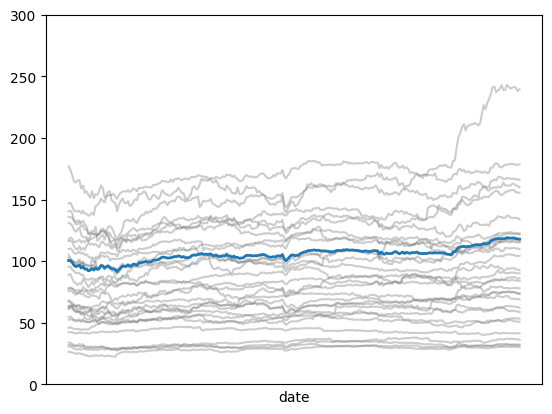
Create a plot showing the symbol and index values over time:
[9]:
import matplotlib
import matplotlib.pyplot as plt

fig, ax = plt.subplots()
price.records.groupby("symbol", observed=True).plot(
    x="date",
    y="value",
    ax=ax,
    alpha=0.4,
    color="grey",
    legend=False,
    ylim=(0, 300),
    xticks=[],
)
index.records.plot(x="date", y="value", ax=ax, linewidth=2, legend=False)
[9]:
<Axes: xlabel='date'>
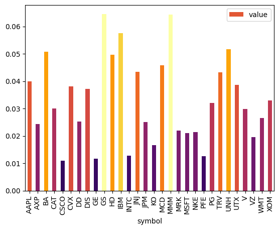
[10]:
sMap = matplotlib.cm.ScalarMappable(
    norm=matplotlib.colors.Normalize(0, weight.records["value"].max()), cmap="inferno"
)
color = [sMap.to_rgba(x) for x in weight.records["value"]]
weight.records.plot.bar(x="symbol", y="value", color=color)
[10]:
<Axes: xlabel='symbol'>
Define dynamic set ds and scalar maxstock:
[11]:
trainingdays = Parameter(m, "trainingdays", records=100)
maxstock = Parameter(m, "maxstock", records=3)
ds = Set(m, "ds", date, description="selected dates")
ds.setRecords(date.records["uni"][:100])
Declaration of the variables and equations used to formulate the optimization model:
[12]:
p = Variable(m, "p", "binary", symbol, description="is stock included?")
w = Variable(m, "w", "positive", symbol, description="what part of the portfolio")
slpos = Variable(m, "slpos", "positive", date, description="positive slack")
slneg = Variable(m, "slneg", "positive", date, description="negative slack")
Defining the actual model#
We now come to the decision problem, where we want to pick a small subset of the stocks together with some weights, such that this portfolio has a similar behavior to our overall Dow Jones index.
The model is based on a linear regression over the time series, but we minimize the loss using the L1-norm (absolute value), and allow only a fixed number of weights to take nonzero values.
\begin{align} \text{minimize} \qquad & \text{obj}:= \sum_{ds} \text{slpos}_{ds} + \text{slneg}_{ds} \\ \text{subject to} \qquad & \sum_{s} \text{price}_{ds, s} \cdot w_{s} = \text{index}_{ds} + \text{slpos}_{ds} - \text{slneg}_{ds} & (\forall{ds}) \\ & w_{s} \leq p_{s} & (\forall{s}) \\ & \sum_{s}{p_{s}} \leq \text{maxstock} \\ & w_{s}\geq 0, \qquad p_{s}\in \{0,1\} & (\forall s) \\ & \text{slpos}_{d}\geq 0, \qquad \text{slneg}_{d}\geq 0 & (\forall d) \end{align}
[13]:
fit = Equation(m, name="deffit", domain=[ds], description="fit to Dow Jones index")
fit[ds] = Sum(s, price[ds, s] * w[s]) == index[ds] + slpos[ds] - slneg[ds]

pick = Equation(
    m, name="defpick", domain=[s], description="can only use stock if picked"
)
pick[s] = w[s] <= p[s]

numstock = Equation(m, name="defnumstock", description="few stocks allowed")
numstock[...] = Sum(s, p[s]) <= maxstock
Objective:
[14]:
obj = Sum(ds, slpos[ds] + slneg[ds])
Model:
[15]:
pickstock = Model(
    container=m,
    name="pickstock",
    equations=m.getEquations(),
    problem="MIP",
    sense=Sense.MIN,
    objective=obj,
)
Specify ‘maxstock’ and ‘trainingdays’ and solve the model:
[16]:
ds.setRecords(date.records["uni"][:100])
maxstock.setRecords(3)
Solve:
[17]:
pickstock.solve(options=Options(relative_optimality_gap=0.01, time_limit=6))
[17]:
| Solver Status | Model Status | Objective | Num of Equations | Num of Variables | Model Type | Solver | Solver Time | |
|---|---|---|---|---|---|---|---|---|
| 0 | Normal | Integer | 45.5725938967286 | 132 | 261 | MIP | CPLEX | 0.142 |
Generate reporting parameters:
[18]:
fund = Parameter(m, "fund", [date], description="Index fund report parameter")
fund[d] = Sum(s, price[d, s] * w.l[s])
error = Parameter(m, "error", [date], description="Absolute error")
error[d] = index[d] - fund[d]
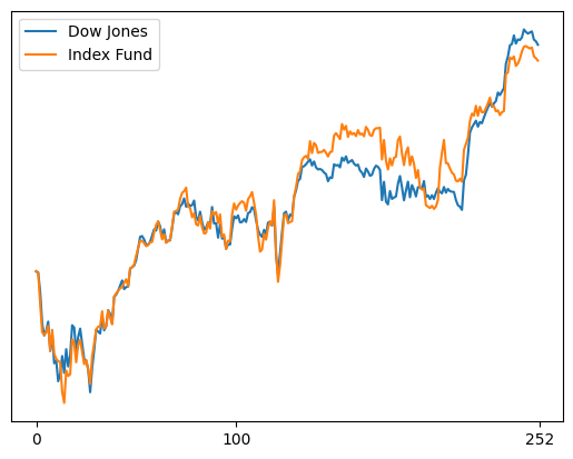
Plotting the results:
[19]:
fig, ax = plt.subplots()
trainingDays = int(trainingdays.records.iloc[0].to_list()[0])
index.records.plot(
    y="value",
    ax=ax,
    xticks=[0, trainingDays, len(date.records)],
    yticks=[],
    label="Dow Jones",
)
fund.records.plot(
    y="value",
    ax=ax,
    xticks=[0, trainingDays, len(date.records)],
    yticks=[],
    label="Index Fund",
)
[19]:
<Axes: >
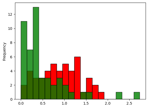
[20]:
maxError = error.records["value"].max()
fig, ax = plt.subplots(edgecolor="black")
error.records["value"][trainingDays:].plot.hist(
    x="date",
    y="value",
    ax=ax,
    bins=20,
    range=(0, maxError),
    label="later",
    color="red",
    edgecolor="black",
)
error.records["value"][:trainingDays].plot.hist(
    x="date",
    y="value",
    ax=ax,
    bins=20,
    range=(0, maxError),
    label="training",
    color="green",
    alpha=0.8,
    edgecolor="black",
)
[20]:
<Axes: ylabel='Frequency'>